Archive for the ‘Machine Learning’ category

sklearn 典型的回归模型

September 14th, 2017

回归模型中线性回归是最最基本的模型,也是在数据处理中运用最多的模型。sklearn提供了一套完备的工具集,可以对数据进行拟合和预测。

from sklearn.model_selection import train_test_split
from sklearn.linear_model import LinearRegression,RidgeCV,LassoCV,ElaticNetCV
from sklearn.preprocessing.PolynomialFeatures import PolynomialFeatures
models = [Pipeline([  
        ('poly', PolynomialFeatures()),  
        ('linear', LinearRegression(fit_intercept=False))]),  
        Pipeline([  
            ('poly', PolynomialFeatures()),  
            ('linear', RidgeCV(alphas=np.logspace(-3, 2, 50), fit_intercept=False))]),  
        Pipeline([  
            ('poly', PolynomialFeatures()),  
            ('linear', LassoCV(alphas=np.logspace(-3, 2, 50), fit_intercept=False))]),  
        Pipeline([  
            ('poly', PolynomialFeatures()),  
            ('linear', ElasticNetCV(alphas=np.logspace(-3, 2, 50), l1_ratio=[.1, .5, .7, .9, .95, .99, 1],  
                                    fit_intercept=False))])  
    ]  

模型中的fit_intercept代表是否存在截距,默认是开启的,normalize:标准化开关,默认关闭。

通过上面的头文件就可以看出来除了提供最最基本的LinearRegression以外,还提供带有L1 L2范数的LassoCV和RidgeCV。

LinearRegression的损失函数为J(θ)=1/2(Xθ−Y)T(Xθ−Y) 。优化方法为梯度下降和最小二乘法,scikit中采用最小二乘
。只要数据线性相关,LinearRegression就是首选,如果发现拟合或者预测的不够好,再考虑其他的线性回归库。

LassoCV的损失函数为J(θ)=1/2m(Xθ−Y)T(Xθ−Y)+α||θ|| 。即 线性回归LineaRegression的损失函数+L1(1范式的正则化项α||θ||) ,Lasso回归可以使得一些特征的系数变小,甚至还使一些绝对值较小的系数直接变为0,从而增强模型的泛化能力,因此对于高维的特征数据,尤其是线性关系是稀疏的,就采用Lasso回归,或者是要在一堆特征里面找出主要的特征。

RidgeCV的损失函数为J(θ)=1/2(Xθ−Y)T(Xθ−Y)+1/2(α||θ||^2)。即线性回归LineaRegression的损失函数+L2(2范式的正则化项1/2(α||θ||^2))),其中a为超参数 alphas=np.logspace(-3, 2, 50) 从给定的超参数a中选择一个最优的,logspace用于创建等比数列 本例中 开始点为10的-3次幂,结束点10的2次幂,元素个数为50.并且从这50个数中选择一个最优的超参数。Ridge回归中超参数a和回归系数θ的关系,a越大,正则项惩罚的就越厉害,得到的回归系数θ就越小,最终趋近与0。如果a越小,即正则化项越小,那么回归系数θ就越来越接近于普通的线性回归系数。
#使用场景:只要数据线性相关,用LinearRegression拟合的不是很好,需要正则化,可以考虑使用RidgeCV回归。

ElaticNetCV的损失函数为J(θ)=1/2m(Xθ−Y)T(Xθ−Y)+αρ||θ||1+α(1−ρ)/2||θ||22 其中α为正则化超参数,ρ为范数权重超参数 。乍一看就是Lasso和Ridge损失函数的合体。其中alphas=np.logspace(-3, 2, 50), l1_ratio=[.1, .5, .7, .9, .95, .99, 1] 。ElasticNetCV会从中选出最优的 a和p 。ElasticNetCV类对超参数a和p使用交叉验证,帮助选择合适的a和p,使用场景:ElasticNetCV类在我们发现用Lasso回归太过(太多特征被稀疏为0),而Ridge回归也正则化的不够(回归系数衰减太慢)的时候。

所以综上排名:LinearRegression > LassoCV(稀疏) >  ElaticNetCV  > RidgeCV(稠密) 

model = models[t]  
model.set_params(poly__degree=d) #设置多项式回归的阶
model.fit(x, y.ravel()) 
lin = model.get_params('linear')['linear'] 
if hasattr(lin, 'alpha_'): 
  ...
if hasattr(lin, 'l1_ratio_'): # 根据交叉验证结果,从输入l1_ratio(list)中选择的最优l1_ratio_(float) 
  ...
print output, lin.coef_.ravel(),lin.intercept_ 
y_hat = model.predict(x_hat)  
s = model.score(x, y)  

sklearn中提供了pipeline,只要把模型定义好,就可以直接利用fit对数据进行拟合,拟合完毕后使用predict进行预测。其中通过get_params可以获取某个模型,然后就能访问该回归模型的coef_和intercept_ ,如果模型设置的fit_intercept=false,那么打印出的lin.coef_中第一项就是截距,后面的为各个相关系数,lin.intercept_为0。如果置为true,那么lin.intercept_为截距值。

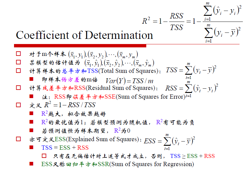
model.score主要用来衡量模型的拟合程度,Returns the coefficient of determination R^2 of the prediction.

R^2就是1-RSS/TSS,R^2越大,拟合效果越好。如果预测值为样本期望,那么R^2为0。

附sklearn工具类

参数列表 类别 fit方法有用 说明
sklearn.preprocessing StandardScaler 特征 无监督 Y 标准化
sklearn.preprocessing MinMaxScaler 特征 无监督 Y 区间缩放
sklearn.preprocessing Normalizer 特征 无信息 N 归一化
sklearn.preprocessing Binarizer 特征 无信息 N 定量特征二值化
sklearn.preprocessing OneHotEncoder 特征 无监督 Y 定性特征编码
sklearn.preprocessing Imputer 特征 无监督 Y 缺失值计算
sklearn.preprocessing PolynomialFeatures 特征 无信息 N 多项式变换(fit方法仅仅生成了多项式的表达式)
sklearn.preprocessing FunctionTransformer 特征 无信息 N 自定义函数变换(自定义函数在transform方法中调用)
sklearn.feature_selection VarianceThreshold 特征 无监督 Y 方差选择法
sklearn.feature_selection SelectKBest 特征/特征+目标值 无监督/有监督 Y 自定义特征评分选择法
sklearn.feature_selection SelectKBest+chi2 特征+目标值 有监督 Y 卡方检验选择法
sklearn.feature_selection RFE 特征+目标值 有监督 Y 递归特征消除法
sklearn.feature_selection SelectFromModel 特征+目标值 有监督 Y 自定义模型训练选择法
sklearn.decomposition PCA 特征 无监督 Y PCA降维
sklearn.lda LDA 特征+目标值 有监督 Y LDA降维

参考

http://scikit-learn.org/stable/modules/generated/sklearn.linear_model.RidgeCV.html

CNN参数小结

May 11th, 2017

CNN(Convolutional Neural Networks)是当下最火的一种神经网络,主要用来识别图像。CNN由三部分组成:Convolutional Layer, Pooling Layer 和 Fully-Connected Layer,卷积层和池化都是CNN特有的,全连接层是传统的神经网络。

整个网络流程就是 [INPUT – CONV – RELU – POOL – FC],其中CONV-RELU-POOL可以添加很多层,如图所示

举个例子:

  • 输入的数据都是28x28x1的图像,意思就是长宽都是28的pixel,并且是单通道图像。
  • 卷积层中,神经元与输入层中的一个局部区域相连,每个神经元都计算自己与输入层相连的小块区域与自己权重的内积。卷积层会计算所有神经元的输出。如果我们使用25个filter[3x3x25],每个filter是得到的输出数据体的维度就是[26x26x25]。
  • ReLU层将会逐个元素地进行激活函数操作,比如使用以0为阈值的max(0,x)作为激活函数。该层对数据尺寸没有改变,还是[26x26x25]。
  • 汇聚层在在空间维度(宽度和高度)上进行降采样(downsampling)操作,其实也就是POOL层[2×2],数据尺寸变为[13x13x25]。
  • 然后可以再次进行卷积、ReLU和Pool。
  • 全连接层将会计算分类评分,数据尺寸变为[1x1x10],其中10个数字对应的就是CIFAR-10中10个类别的分类评分值,全连接层与常规神经网络一样,其中每个神经元都与前一层中所有神经元相连接。

最开始卷积的维度变化让我很头疼,看了好久才理解。总结下面公式:

  • 输入数据体的尺寸为W1 * H1 * D1
  • 4个参数:
    filter的数量K
    filter的空间尺寸F
    步长stride S
    零填充数量(the amount of zero padding)P
  • 输出数据体的尺寸为W2 * H2 * D2 ,其中:
    W2=(W1-F+2P)/S+1
    H2=(H1-F+2P)/S+1 (宽度和高度的计算方法相同)
    D2=K
    由于参数共享,每个滤波器包含F * F *D1个权重,卷积层一共有F * F * D1  K个权重和K个偏置。

每进行一次卷积,图像的深度就增加一倍,深度与filter的数量K紧密相关!

常见的设置是F=3,S=1,P=1,零填充数量就是为了让输入图像长宽变为偶数(其实就是在图像外围填充0),例如是32、64、128等,而使用S=1的步长,是因为使得空间维度的降采样全部由Pooling层负责,卷积层只负责对输入数据体的深度进行变换。

使用这些参数需要考虑到内存的占用率,比如使用64个尺寸为3×3的滤波器对【224x224x3】的图像进行卷积,零填充为1,步长为1,那么得到的激活数据体尺寸是[224x224x64]。这个数量就是一千万的数据特征,或者就是72MB的内存!

第二次池化后,使用Flatten,压扁这个数据集合,建立二层全连接网络,第一层神经元数100,第二层为10。


参考:

http://cs231n.github.io/convolutional-networks/

http://cs231n.stanford.edu/syllabus.html

http://cs.stanford.edu/people/karpathy/convnetjs/demo/cifar10.html

主成分分析(Principal components analysis)的计算过程

April 28th, 2017

今天使用Octave练习计算PCA,发现自己对于这个计算还不是特别了解,特此记录。

首先从txt中获取数据,然后将矩阵都入到X中。

octave:7> data = load('ex2data.txt')
data =

   2.50000   2.40000
   0.50000   0.70000
   2.20000   2.90000
   1.90000   2.20000
   3.10000   3.00000
   2.30000   2.70000
   2.00000   1.60000
   1.00000   1.10000
   1.50000   1.60000
   1.10000   0.90000
octave:8> X = data(:, [1, 2]);
octave:15> mu=mean(X)
mu =

   1.8100   1.9100

求x平均值,然后对于所有的样例,都减去对应的均值。这里x的均值是1.81和1.91,那么一个样例减去均值后即为(0.69,0.49),得到

octave:16> X_norm = bsxfun(@minus, X, mu);
octave:17> X_norm 
X_norm =

   0.690000   0.490000
  -1.310000  -1.210000
   0.390000   0.990000
   0.090000   0.290000
   1.290000   1.090000
   0.490000   0.790000
   0.190000  -0.310000
  -0.810000  -0.810000
  -0.310000  -0.310000
  -0.710000  -1.010000

我们使用这个矩阵去构造协方差矩阵sigma = (X_norm’ * X_norm)/size(X_norm(:,1))

octave:34> sigma = X_norm' * X_norm
sigma =

   5.5490   5.5390
   5.5390   6.4490

octave:35> sigma = sigma/10
sigma =

   0.55490   0.55390
   0.55390   0.64490

使用octave中的svd函数直接计算出协方差的特征值和特征向量

octave:36> [U,S,V] = svd(sigma)
U =

  -0.67787  -0.73518
  -0.73518   0.67787

S =

Diagonal Matrix

   1.155625          0
          0   0.044175

V =

  -0.67787  -0.73518
  -0.73518   0.67787

U为特征向量,S为sigma的特征值,通过特征值可以求变量的retained(保留程度)。
比如此时我们想把2维数据转换到1维数据上,那么可以使用U的第一列或者第二列,通过公式z=U’ * X_norm或者X_norm * U得到降维后的数据。

octave:39> z = X_norm*U(:,1)
z =

  -0.827970
   1.777580
  -0.992197
  -0.274210
  -1.675801
  -0.912949
   0.099109
   1.144572
   0.438046
   1.223821

研究其数理意义,就是求源数据到向量基z的投影误差最小,找到合适的基向量代表这个平面。
http://www.cnblogs.com/jerrylead/archive/2011/04/18/2020209.html

http://www.cnblogs.com/LeftNotEasy/archive/2011/01/19/svd-and-applications.html

修正Neural Network参数小结

April 14th, 2017

在实际构建神经网络的过程中,经常碰到一些选择的问题,现在进行总结:

  • Getting more training examples: Fixes high variance
  • Trying smaller sets of features: Fixes high variance
  • Adding features: Fixes high bias
  • Adding polynomial features: Fixes high bias
  • Decreasing λ: Fixes high bias
  • Increasing λ: Fixes high variance.

当遇到高差异性时(high variance),可以试图增加训练样本或者减少特征数量来解决,但是如果遇到高偏见性(high bias),那么就表明这个训练集可能特征数太少,需要增加特征。λ作为惩罚系数存在,λ越大,惩罚系数越大,越可以修正高差异性,反之修正高偏见性。对于λ的取值,一般遵循在cross-validation set中取最优来决定。

Diagnosing Neural Networks

  • A neural network with fewer parameters is prone to underfitting. It is also computationally cheaper.
  • A large neural network with more parameters is prone to overfitting. It is also computationally expensive. In this case you can use regularization (increase λ) to address the overfitting.

Using a single hidden layer is a good starting default. You can train your neural network on a number of hidden layers using your cross validation set. You can then select the one that performs best.只有一层的神经网络最简单,但是同时可能会造成性能损失,所以我们要增加隐藏层数和特征数,但是复杂的神经网络又会导致过拟合和计算复杂度太高的问题,所以要权衡这种平衡。

Model Complexity Effects:

  • Lower-order polynomials (low model complexity) have high bias and low variance. In this case, the model fits poorly consistently.
  • Higher-order polynomials (high model complexity) fit the training data extremely well and the test data extremely poorly. These have low bias on the training data, but very high variance.
  • In reality, we would want to choose a model somewhere in between, that can generalize well but also fits the data reasonably well.

默认将数据集分为3部分,60%的训练集,20%的cross-validation set和20%的测试集。

参考:

https://www.coursera.org/learn/machine-learning/supplement/llc5g/deciding-what-to-do-next-revisited

http://www.cnblogs.com/sddai/p/5696834.html

How to elaborate and train a Neural Network

March 31st, 2017

Elaborate a Neural Network

First, pick a network architecture; choose the layout of your neural network, including how many hidden units in each layer and how many layers in total you want to have.

  • Number of input units = dimension of features x(i)

  • Number of output units = number of classes

  • Number of hidden units per layer = usually more the better (must balance with cost of computation as it increases with more hidden units)

  • Defaults: 1 hidden layer. If you have more than 1 hidden layer, then it is recommended that you have the same number of units in every hidden layer.

构建 Neural Network 首先要明确要创建几个隐藏层,每个隐藏层有多少个参数。

首先输入单元个数就是输入的特征数,输出的个数就是分类的个数,每个隐藏层中单元的个数是多少?

通常意义上,隐藏层中单元的个数越多,这个分类效果越好,但是需要权衡计算与特征数的关系。默认情况,一个神经网络会存在一个隐藏层,当多余一个隐藏层的情况下,每层拥有的单元个数相同。

Training a Neural Network

  • Randomly initialize the weights
  • Implement forward propagation to get hΘ(x(i)) for any x(i)
  • Implement the cost function
  • Implement backpropagation to compute partial derivatives
  • Use gradient checking to confirm that your backpropagation works. Then disable gradient checking.
  • Use gradient descent or a built-in optimization function to minimize the cost function with the weights in theta.

输入的特征的权重是随机指定的(如果全部输入的权重都为一个常数,那么输入到隐藏层的值就是相同的,那么导致hΘ(x(i))也是相同的,导致symmetry。不同的初始权重就是为了Symmetry Breaking)。

实现前馈传播算法,计算出每层的x(i),实现代价函数,通过反向传播算法计算每个Θ的偏导,然后通过梯度检查测试反向传播算法是否成功,然后将梯度检查disable掉(梯度检查计算复杂度太高)。

最后使用梯度下降找到最小的代价函数值和Θ。这个就是需要的特征集。

参考:

http://blog.csdn.net/jinlianjingd/article/details/50767743

https://www.coursera.org/learn/machine-learning/supplement/Uskwd/putting-it-together